Introduction

If you’ve been reading our blog regularly, you have noticed that we mention decision trees as a modeling tool and have seen us use a few examples of them to illustrate our points. This month, we’ve decided to go more in depth on decision trees—below is a simplified, yet comprehensive, description of what they are, why we use them, how we build them, and why we love them. (Does that make us the tree-huggers of the digital age? Maybe!)

What is a Decision Tree?

A decision tree is a popular method of creating and visualizing predictive models and algorithms. You may be most familiar with decision trees in the context of flow charts. Starting at the top, you answer questions, which lead you to subsequent questions. Eventually, you arrive at the terminus which provides your answer.

Decision trees tend to be the method of choice for predictive modeling because they are relatively easy to understand and are also very effective. The basic goal of a decision tree is to split a population of data into smaller segments. There are two stages to prediction. The first stage is training the model—this is where the tree is built, tested, and optimized by using an existing collection of data. In the second stage, you actually use the model to predict an unknown outcome. We’ll explain this more in-depth later in this post.

It is important to note that there are different kinds of decision trees, depending on what you are trying to predict. A regression tree is used to predict continuous quantitative data. For example, to predict a person’s income requires a regression tree since the data you are trying to predict falls along a continuum. For qualitative data, you would use a classification tree. An example would be a tree that predicts a person’s medical diagnosis based on various symptoms; there are a finite number of target values or categories. It would be tempting to simply conclude that if the information you are trying to predict is a number, it is always a regression tree, but this is not necessarily the case. Zip code is a good example. Despite being a number, this is actually a qualitative measure because zip codes are not calculated; they represent categories.

Key Terms

Before we cover the more complex aspects of decision trees, let’s examine some key terms that will be used in this post. It is important to note that there are multiple terms used to describe these concepts–however, these are the ones that we use at Aunalytics, and we will use these for the duration of this blog post for consistency. However, the alternate terms will be noted as well, in case you encounter them in a different context.

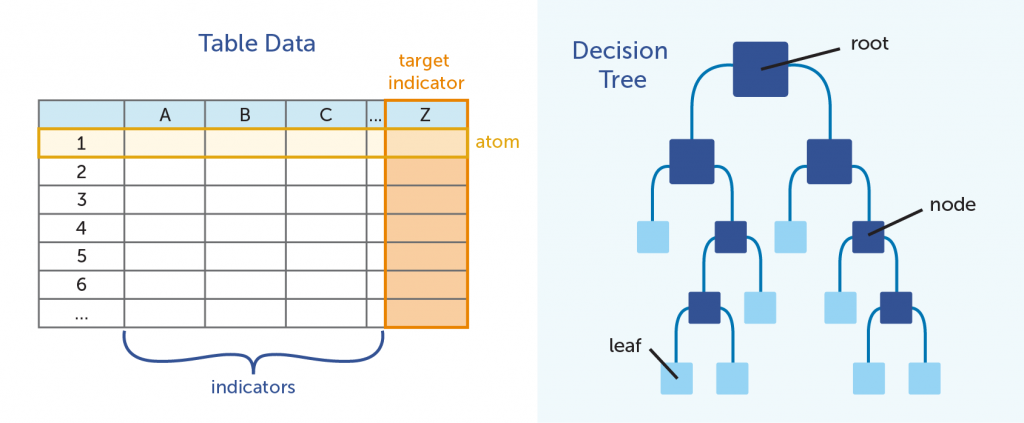
In the table above, Column Z is the target indicator; the piece of information that is being predicted by the model. All modeling is with regards to these data points. Alternate terms: class, predicted variable, target variable

The data in columns A, B, C, and so on are called indicators. The indicators are the data points that are used to to make predictions. Alternate terms: feature, dimension, variable
As a whole, the total collection of indicators forms an indicator vector. Alternate terms: measurement vector, feature vector, dataset

Rows 1, 2, and 3 represent what we refer to as atoms. Each row contains data points as they relate to a singular entity; in our analyses, typically this is an individual person or product. We talked about the atom in a previous blog post.  Alternate terms: instances, examples, data points

Unlike a tree you would see outside your window, decision trees in predictive analytics are displayed upside down. The root of the tree is on top, with the branches going downward.

Each split in the branch, where we break the large group into progressively smaller groups by posing an either-or scenario, is referred to as a node. The a terminal node is called a leaf.

Methodology

As mentioned previously, building a predictive model involves first training the model (and building the tree) by using known data and verifying its accuracy and reliability by using the model on test data that had been set aside to predict the known test outcomes. In the diagram below, the model is initially built using 6 months’ worth of data (the 6th month is the target indicator, and the five months before that are used to train the model that will predict the 6th month’s outcome). The model is evaluated for accuracy and optimized by using the previous month’s data to predict the known outcome for today (a known value). Finally, the model can be used to predict outcomes in the future.

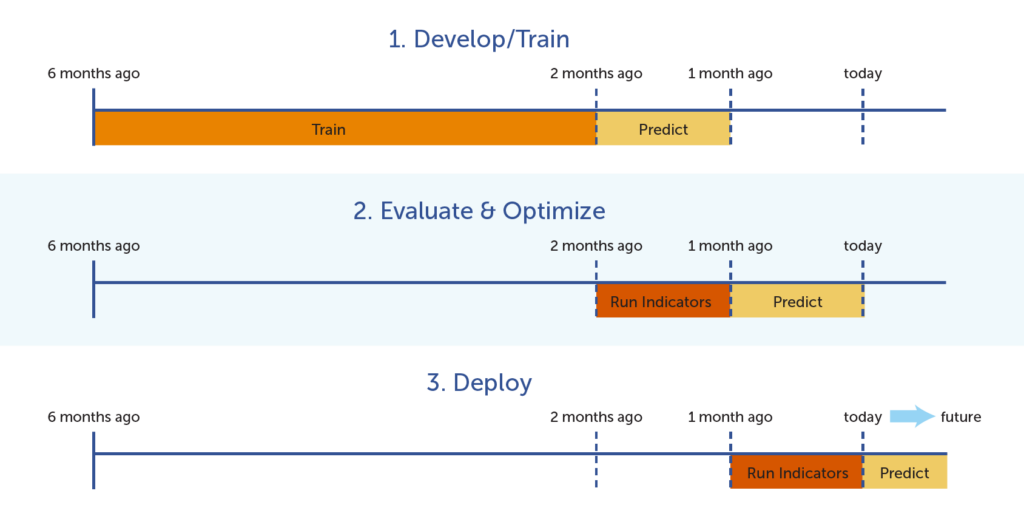
Once the tree has been tested and optimized, it can be used to predict unknown or future outcomes.

Development

When it comes to actually building a decision tree, we start at the root, which includes the total population of atoms. As we move down the tree, the goal is to split the total population into smaller and smaller subsets of atoms at each node; hence the popular description, “divide and conquer.” Each subset should be as distinct as possible in terms of the target indicator. For example, if you are looking at high- vs. low-risk customers, you would want to split each node into two subsets; one with mostly high-risk customers, and the other with mostly low-risk customers.

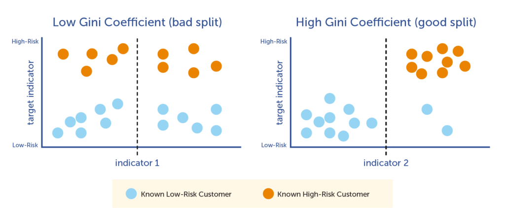
This goal is achieved by iterating through each indicator as it relates to the target indicator, and then choosing the indicator that best splits the data into two smaller nodes. As the computer iterates through each indicator-target pair, it calculates the Gini Coefficient, which is a mathematical calculation that is used to determine the best indicator to use for that particular split. The Gini Coefficient is a score between 0 and 1, with 1 being the best split, and 0 being the worst. The computer chooses the indicator that has the highest Gini Coefficient to split the node, and then moves on to the next node and repeats the process.

In the following illustration, you can see how the graph on the right, showing indicator 1 in terms of the target indicator, is not an optimal split. There are almost equal amounts of both high- and low-risk customers on each side of the split line. However, the graph on the left shows a very good indicator; the line splits the high- and low-risk customers very accurately.

How to calculate a predictive score

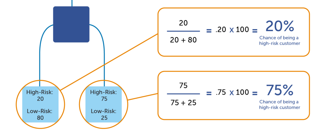
Once the computer program has finished building the tree, predictive scores can be calculated. The predictive score is a percentage of the target indicator in the terminal node (or leaf) of the trained model. In the example below, there are 20 high-risk customers and 80 low-risk customers in the leaf to the far left. Any atom that ends up in the left leaf would be said to have a 20% chance of being a high-risk customer (20 / (20 + 80) = 20%). But for the leaf on the right, a customer would have a 75% chance of being a high-risk customer (75 / (75 + 25) = 75%). This demonstrates that a model can predict whether certain atoms have a higher propensity to a target indicator. It is important to remember that it is a prediction, which is not 100% accurate (we’re not psychics!) However, it’s a much more accurate than a random guess, which is enough to make a huge difference!

Optimizing the Model

How to reduce bias

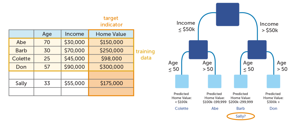
There is one major potential pitfall when working with decision trees, and that is creating an overly-complex tree. With decision trees, simplicity is the key to reducing bias. If a tree grows too large, it ceases to be useful. The image below illustrates this point with a very simplified example. As you can see, the model splits the data in such a way that the bottom leaves only have one person each. All this tree does is show the information in the table in a new way. It adds no additional insight; it only restates the data. You will also notice that the tree is fairly inaccurate; if you add Sally’s data to the mix, you see that it predicts that she has a much more expensive home value than she actually does. The tree has failed to allow for novel circumstances outside of the training data. This is known as overfitting (or overlearning).

The challenge, then, is to create a tree that is specific enough to allow for actionable insights, yet not complex to the point where it does not give any new information or allow for possibilities that were not expressly stated in the data. This problem is alleviated through a process known as pruning.

The idea behind pruning is to build a very complex tree, and then take away enough levels of complexity until it is as simple as possible, yet still maximally accurate in predicting the target indicator. This is done by employing a simple technique that was mentioned earlier in this post: set aside a portion of the training data to be used as validation data. Since this data was not used to train the model, it will show whether or not the decision tree has overlearned the training data. If the predictive accuracy (also known as lift) with the test data are low, the size of the tree is reduced, and the process is repeated until the tree reaches the sweet spot between high accuracy and low complexity.

How to knock it out of the park

By now, you’ve learned how decision trees are built to ensure accuracy of results, while avoiding overfitting. But how do data scientists take a predictive model to the next level? Use multiple models! When multiple models are combined into a single mega-model, it is referred to as an ensemble model. Using an ensemble of predictive models can improve upon a single model’s performance by anywhere from 5-30%. That’s huge! There are a few ways of creating an ensemble, but we will discuss two common methods: bagging and random forests.

Bagging is a shortened version of the term “bootstrap aggregating.” In this method, the training data is split into smaller subsets of data, and within the subsets, some atoms are randomly duplicated or removed. This ensures that no single atom disproportionately affects the final results. A decision tree is created for each subset, and the results of each tree are combined. By combining these trees into an ensemble model, the shortcomings of any single tree are overcome.

Random forests are closely related to bagging, but add an extra element: instead of only randomizing the atoms in the various subsets of data, it also randomly duplicates or deletes indicators. If a certain indicator is flawed or shows a false correlation with the target indicator, it is overcome by the fact that the flawed indicator is not present in certain trees, or is reduced in importance in others.

Conclusion

Hopefully now you have a better understanding of decision trees; why they are used frequently in predictive modeling, how they are created, and how they can be optimized for best results. Decision trees are a powerful tool for data scientists, but they must be handled with care. Although much of the repetitive tasks are achieved by use of computers (hence the term machine learning), all aspects of the process must be orchestrated and overseen by an experienced data scientist in order to create the most accurate model. But the work is well worth the effort in the end when an accurate model leads to actionable insights.

Note: If you are interesting in learning more about decision trees and predictive modeling, we would recommend the book Predictive Analytics by Eric Siegel, or the article “How to Grow and Prune a Classification Tree” by David Austin (which goes into greater detail on the mathematical explanations).