
Building a Data Warehouse
To perform interesting predictive or historical analysis of ever-increasing amounts of data, you first have to make it small. In our business, we frequently create new, customized datasets from customer source data in order to perform such analysis. The data may already be aggregated, or we may be looking at data across disparate data sources. Much time and effort is spent preparing this data for any specific use case, and every time new data is introduced or updated, we must build a cleaned and linked dataset again.
To streamline the data preparation process, we’ve begun to create data warehouses as an intermediary step; this ensures that the data is aggregated into a singular location and exists in a consistent format. After the data warehouse is built, it is much easier for our data scientists to create customized datasets for analysis, and the data is in a format that less-technical business analysts can query and explore.
Data warehouses are not a new concept. In our last blog post, we talked about the many reasons why a data warehouse is a beneficial method for storing data to be used for analytics. In short, a data warehouse can improve the efficiency of our process by creating a structure for aggregated data and allows data scientists and analysts to more quickly get the specific data they need for any analytical query.
A data warehouse is defined by its structure and follows these four guiding principles:
- Subject-oriented: The structure of a data warehouse is centered around a specific subject of interest, rather than as a listing of transactions organized by timestamps.
- Integrated: In a data warehouse, data from multiple sources is integrated into a single structure and consistent format.
- Non-volatile: A data warehouse is a stable system; it is not constantly changing.
- Time-variant: The term “time-variant” refers to the inclusion of historical data for analysis of change over time.
These principles underlie the data warehouse philosophy, but how does a data warehouse work in practice? We will explore two of the more concrete aspects of a data warehouse: how the data is brought into the warehouse, and how the data may be structured once inside.
Data Flow into a Warehouse
Most companies have data in various operational systems; marketing databases, sales databases, and even external data purchased from vendors. They may even have a data warehouse of their own for certain areas of their business. Unfortunately, it is next to impossible to directly compare data across various locations. In order to do such analysis, a great amount of effort is needed to get the data onto a common platform and into a consistent format.
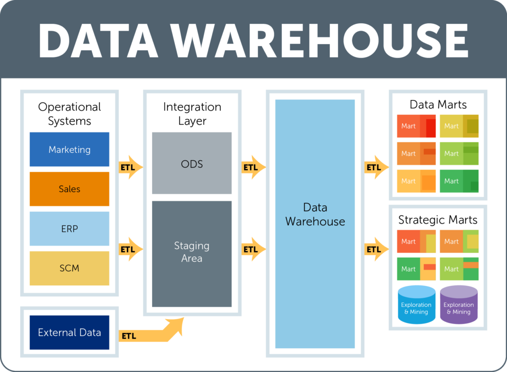
First, these disparate data sources must be combined into a common location. The data is initially brought to an area known as the integration layer. Within the integration layer, there is an ODS (operational data store) and a staging area, which work together (or independently at times) to hold, transform, and perform calculations on data prior to the data being added to the data warehouse layer. This is where the data is organized and put into a consistent format.
Once the data is loaded into the data warehouse (the structure of which we will discuss later on in the blog post), it can be accessed by users through a data mart. A data mart is a subset of the data that is specific to individual department or users and includes only the data that is most relevant to their specific use cases. There can be multiple data marts, but they all pull from the same data warehouse to ensure that the information that is seen is the most up-to-date and accurate. Many times, in addition to marts, a data warehouse will have databases specially purposed for exploration and mining. A data scientist can explore the data in the warehouse this way, and generate custom datasets on an analysis-by-analysis basis.
At every step of the way, moving the data from one database to another involves using a series of operations known as ETL, which stands for extract, transform, and load. First, the data must be extracted from the original source. Next, that data is transformed into a consistent format, and finally, the data is loaded into the target database. These actions are performed in every step of the process.
Data Warehouse Structure
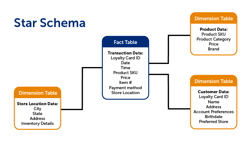
There are a few different ways that the data within the warehouse can be structured. A common way to organize the data is to use what is called a star schema. A star schema is composed of two types of tables: fact tables and dimension tables.
Fact tables contain data that corresponds to a particular business practice or event. This would include transaction details, customer service requests, or product returns, to name a few. The grain is the term for the level of detail of the fact table. For instance, if your fact table recorded transaction details, does each row include the detail of the transaction as a whole, or each individual item that was purchased? The latter would have a more detailed grain.
While fact tables include information on specific actions, a dimension table, on the other hand, includes non-transactional information that relates to the fact table. These are the items of interest in analytics: data on each individual customer, location/branch, employee, product, etc. In other words, the dimension is the lens through which you can examine and analyze the fact data.
There are typically far fewer facts, which are “linked” to the various dimension tables, forming a structure that resembles a star, hence the term star schema.
A snowflake schema is similar to the star schema. The main difference is that in a snowflake schema, the dimension tables are normalized--that means that the individual dimension tables from the star schema are re-organized into a series of smaller, sub-dimension tables which reduces data redundancy. This is done so that the same information isn’t stored in multiple tables, which makes it easier to change or update the information since it only has to be change in one location. The downside of the snowflake schema is that it can be complicated for users to understand, and requires more code to generate a report. Sometimes it is best to maintain a de-normalized star schema for simplicity’s sake.
Conclusion
These are just the basics of how data flows into a data warehouse, and how a warehouse could be structured. While the star and snowflake schemas are not the only way (there is also a newer schema called a Data Vault), they do provide a standardized way to store and interact with historical data. Ultimately, a well-organized data warehouse allows data scientists and analysts to more easily explore data, ask more questions, and find the answers they need in a more timely fashion.
Why Using a Data Warehouse Optimizes Analytics
Beginning an analytics project is no small task. After choosing the initial question to be answered and formulating a plan of actions to be taken as a result, the next logical step is to complete an inventory of the available data sources and determine what data is needed to reach the decided-upon analysis goal.
It’s common for a company to have many different databases containing a wide variety of information. To gain a complete view of of a company through analytics, data from many sources is aggregated to one place. A company may have transaction data in one database, customer information in another, and website activity logs in yet another. Bringing all of this data together is a critical part of any analytics project; however, it poses two major challenges.
The first challenge: data is messy. When aggregating data from different sources, the formatting of data points is frequently inconsistent, data may be missing from multiple fields, or the databases may have completely different schemas. In order to build any kind of predictive model or historical analysis, data must be cleaned and organized. This process can be very difficult and time consuming.
The second challenge: analytics requires hardware and software that is powerful and flexible. Most business people have experience running reports and looking at short-term trends. However, data scientists are looking at the bigger picture. They may be sifting through months, or even years, worth of data to uncover trends.
This means that for an analytics project, the data must be stored in a system that has the ability and computing power to comb through thousands of rows of data. The system must also allow data scientists and analysts the flexibility to run a wide variety of queries. Advanced analytics is a journey of discovery; the question being answered may evolve over time as new trends are discovered. Each inquiry leads to new questions as the company journeys deeper into analytics.
Because of these constraints, it is important to consider the physical and virtual structure surrounding the data. Setting up the most efficient structure for the job at hand is the best way to optimize any project. We will go through two ways to manage data for analytics:
One Way to Do It
Data cleaning and linking is time-consuming. In the interest of time, it may seem that the quickest way to get a desired answer is to prepare only the data that is actually needed for a given analysis. Data scientists spend large amounts of time preparing the data, so why waste time aggregating, cleaning and linking data that won’t be used?
Because analytics never stops at a single question and answer (and, as software engineers know, requirements often change many times before the final product is released), a project-specific cleaned and linked dataset may need to be altered many times. A subsequent or new question may involve the use of additional or completely different data points. The relevant data must be cleaned, linked, and organized from the source databases all over again. This especially becomes an issue when the question at hand requires the most up-to-date information. Each time new data is included, the dataset must be updated or completely re-generated and linked. Think of how many new, ad hoc datasets would be created from source data over the lifetime of the analytics project!
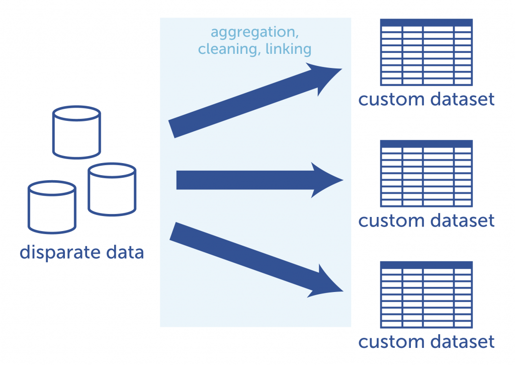
Each analytics project requires a new custom dataset to be created from
the source databases. This requires time and effort to achieve.
A Better Way
It is important to think of the bigger picture when it comes to data analysis. It is highly unlikely that an analyst or data scientist will ever stop with one question. So, instead of creating specialized datasets for analysis on an ad hoc basis, it is more efficient in the long run to create an integrated, linked, and cleaned data warehouse to house the entirety of the data. From there, a data scientist or analyst can build custom datasets for their analyses. Because the data is pre-cleaned and stored in an organized manner, it is relatively simple for a data scientist or analyst to select the pieces of information needed to create an analytics-ready dataset on the fly.
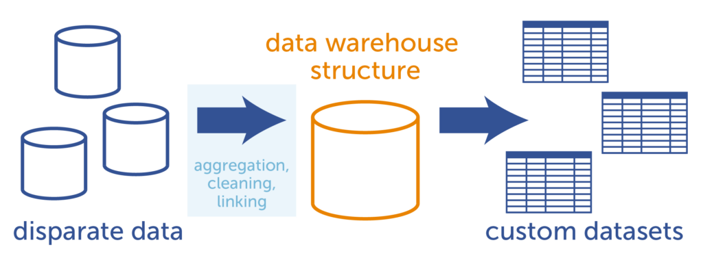
With a data warehouse, the disparate data is aggregated, cleaned, and linked into a single database structure.
From there, custom datasets for analytics are generated more easily.
Data Warehouse vs. Transactional Databases
The term “data warehouse” refers to a philosophy on creating a relational database system that is optimized for query operations and analyses. This differs from other database systems in a number of ways.
Most organizations that are collecting data have at least one (and sometimes many) online transaction processing (OLTP) databases. An OLTP database is used to collect transactional data, and is designed to work well when new records are added frequently, in real time. An example would be a database that collects website click information, or logs every time a customer makes a purchase. These databases give users the ability to perform only a few, set operations because the majority of the computing workload is devoted to recording new transactions in real-time. To keep an OLTP database at top speed, older data is frequently archived. Since analytics requires historical data and the ability to run a variety of exploratory operations on the data, this is not the ideal type of environment for an analysis to occur.
A data warehouse, on the other hand, is focused on analysis rather than recording data in real-time. This give the analyst or data scientist the computing power and flexibility needed to explore historical data to find deeper trends.
There are four guiding principles for data warehouse systems, as defined by the father of data warehousing, William Inmon:
- Subject-oriented: The structure of a data warehouse is centered around a specific subject of interest, rather than as a listing of transactions organized by timestamps. For instance, a data warehouse might have the transactions organized, instead, by the customer who made the transaction. (This would be what we call an “atom-centric” view, with the customer as an atom.) An analyst or data scientist can look for trends in customer transactions over time, and draw comparisons between similar customers and their transaction histories.
- Integrated: In a data warehouse, data from multiple sources is integrated into a single structure and consistent format. In the process of integration, naming conflicts are resolved, units of measure are converted into a consistent format, and missing data may be replaced.
- Non-volatile: A data warehouse is a stable system. Unlike an OLTP database, data is not constantly being added or changed.
- Time-variant: The term “time-variant” refers to the inclusion of historical data for analysis of change over time. Since a data warehouse includes all data rather than just a snapshot of the most recent transactions, a data scientist can begin to search long-term trends.
As you can see, there are many benefits to using a data warehousing system for analytics. The idea was conceived with analytics in mind, and this type of database structure can speed the time to insights, especially when pursuing subsequent analytics projects. A data warehouse allows data scientists and analysts to spend more time deeply exploring the data, rather than wasting precious hours on data preparation.
Conclusion
Building a data warehouse is the best long-term solution for an advanced analytics program. But how does a data warehouse work, and how to data scientists go about building them? Stay tuned. In a future blog post, we will discuss some of the more technical aspects of data warehouses: how they are built and updated; and the various ways to structure the data to optimize analytics.
Decision Trees: An Overview
Introduction
If you’ve been reading our blog regularly, you have noticed that we mention decision trees as a modeling tool and have seen us use a few examples of them to illustrate our points. This month, we’ve decided to go more in depth on decision trees—below is a simplified, yet comprehensive, description of what they are, why we use them, how we build them, and why we love them. (Does that make us the tree-huggers of the digital age? Maybe!)
What is a Decision Tree?
A decision tree is a popular method of creating and visualizing predictive models and algorithms. You may be most familiar with decision trees in the context of flow charts. Starting at the top, you answer questions, which lead you to subsequent questions. Eventually, you arrive at the terminus which provides your answer.
Decision trees tend to be the method of choice for predictive modeling because they are relatively easy to understand and are also very effective. The basic goal of a decision tree is to split a population of data into smaller segments. There are two stages to prediction. The first stage is training the model—this is where the tree is built, tested, and optimized by using an existing collection of data. In the second stage, you actually use the model to predict an unknown outcome. We’ll explain this more in-depth later in this post.
It is important to note that there are different kinds of decision trees, depending on what you are trying to predict. A regression tree is used to predict continuous quantitative data. For example, to predict a person’s income requires a regression tree since the data you are trying to predict falls along a continuum. For qualitative data, you would use a classification tree. An example would be a tree that predicts a person’s medical diagnosis based on various symptoms; there are a finite number of target values or categories. It would be tempting to simply conclude that if the information you are trying to predict is a number, it is always a regression tree, but this is not necessarily the case. Zip code is a good example. Despite being a number, this is actually a qualitative measure because zip codes are not calculated; they represent categories.
Key Terms
Before we cover the more complex aspects of decision trees, let’s examine some key terms that will be used in this post. It is important to note that there are multiple terms used to describe these concepts--however, these are the ones that we use at Aunalytics, and we will use these for the duration of this blog post for consistency. However, the alternate terms will be noted as well, in case you encounter them in a different context.
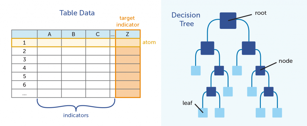
In the table above, Column Z is the target indicator; the piece of information that is being predicted by the model. All modeling is with regards to these data points. Alternate terms: class, predicted variable, target variable
The data in columns A, B, C, and so on are called indicators. The indicators are the data points that are used to to make predictions. Alternate terms: feature, dimension, variable
As a whole, the total collection of indicators forms an indicator vector. Alternate terms: measurement vector, feature vector, dataset
Rows 1, 2, and 3 represent what we refer to as atoms. Each row contains data points as they relate to a singular entity; in our analyses, typically this is an individual person or product. We talked about the atom in a previous blog post. Alternate terms: instances, examples, data points
Unlike a tree you would see outside your window, decision trees in predictive analytics are displayed upside down. The root of the tree is on top, with the branches going downward.
Each split in the branch, where we break the large group into progressively smaller groups by posing an either-or scenario, is referred to as a node. The a terminal node is called a leaf.
Methodology
As mentioned previously, building a predictive model involves first training the model (and building the tree) by using known data and verifying its accuracy and reliability by using the model on test data that had been set aside to predict the known test outcomes. In the diagram below, the model is initially built using 6 months’ worth of data (the 6th month is the target indicator, and the five months before that are used to train the model that will predict the 6th month’s outcome). The model is evaluated for accuracy and optimized by using the previous month’s data to predict the known outcome for today (a known value). Finally, the model can be used to predict outcomes in the future.
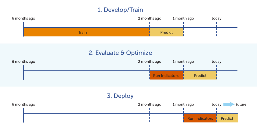
Once the tree has been tested and optimized, it can be used to predict unknown or future outcomes.
Development
When it comes to actually building a decision tree, we start at the root, which includes the total population of atoms. As we move down the tree, the goal is to split the total population into smaller and smaller subsets of atoms at each node; hence the popular description, “divide and conquer.” Each subset should be as distinct as possible in terms of the target indicator. For example, if you are looking at high- vs. low-risk customers, you would want to split each node into two subsets; one with mostly high-risk customers, and the other with mostly low-risk customers.
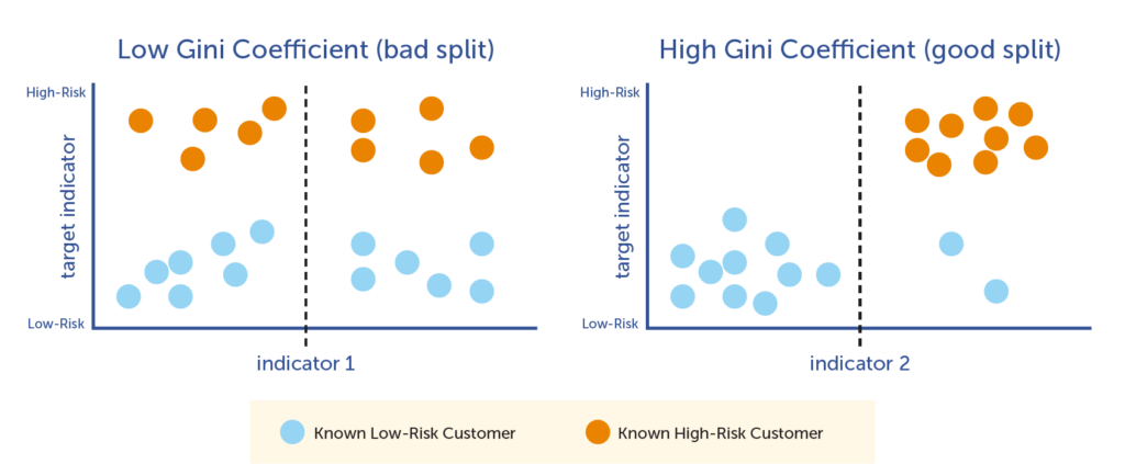
This goal is achieved by iterating through each indicator as it relates to the target indicator, and then choosing the indicator that best splits the data into two smaller nodes. As the computer iterates through each indicator-target pair, it calculates the Gini Coefficient, which is a mathematical calculation that is used to determine the best indicator to use for that particular split. The Gini Coefficient is a score between 0 and 1, with 1 being the best split, and 0 being the worst. The computer chooses the indicator that has the highest Gini Coefficient to split the node, and then moves on to the next node and repeats the process.
In the following illustration, you can see how the graph on the right, showing indicator 1 in terms of the target indicator, is not an optimal split. There are almost equal amounts of both high- and low-risk customers on each side of the split line. However, the graph on the left shows a very good indicator; the line splits the high- and low-risk customers very accurately.
How to calculate a predictive score
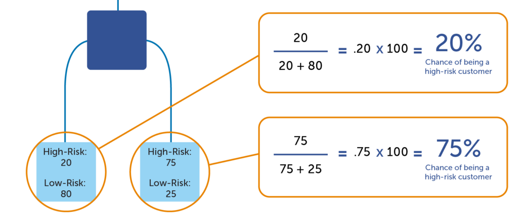
Once the computer program has finished building the tree, predictive scores can be calculated. The predictive score is a percentage of the target indicator in the terminal node (or leaf) of the trained model. In the example below, there are 20 high-risk customers and 80 low-risk customers in the leaf to the far left. Any atom that ends up in the left leaf would be said to have a 20% chance of being a high-risk customer (20 / (20 + 80) = 20%). But for the leaf on the right, a customer would have a 75% chance of being a high-risk customer (75 / (75 + 25) = 75%). This demonstrates that a model can predict whether certain atoms have a higher propensity to a target indicator. It is important to remember that it is a prediction, which is not 100% accurate (we’re not psychics!) However, it’s a much more accurate than a random guess, which is enough to make a huge difference!
Optimizing the Model
How to reduce bias
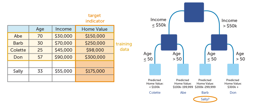
There is one major potential pitfall when working with decision trees, and that is creating an overly-complex tree. With decision trees, simplicity is the key to reducing bias. If a tree grows too large, it ceases to be useful. The image below illustrates this point with a very simplified example. As you can see, the model splits the data in such a way that the bottom leaves only have one person each. All this tree does is show the information in the table in a new way. It adds no additional insight; it only restates the data. You will also notice that the tree is fairly inaccurate; if you add Sally’s data to the mix, you see that it predicts that she has a much more expensive home value than she actually does. The tree has failed to allow for novel circumstances outside of the training data. This is known as overfitting (or overlearning).
The challenge, then, is to create a tree that is specific enough to allow for actionable insights, yet not complex to the point where it does not give any new information or allow for possibilities that were not expressly stated in the data. This problem is alleviated through a process known as pruning.
The idea behind pruning is to build a very complex tree, and then take away enough levels of complexity until it is as simple as possible, yet still maximally accurate in predicting the target indicator. This is done by employing a simple technique that was mentioned earlier in this post: set aside a portion of the training data to be used as validation data. Since this data was not used to train the model, it will show whether or not the decision tree has overlearned the training data. If the predictive accuracy (also known as lift) with the test data are low, the size of the tree is reduced, and the process is repeated until the tree reaches the sweet spot between high accuracy and low complexity.
How to knock it out of the park
By now, you’ve learned how decision trees are built to ensure accuracy of results, while avoiding overfitting. But how do data scientists take a predictive model to the next level? Use multiple models! When multiple models are combined into a single mega-model, it is referred to as an ensemble model. Using an ensemble of predictive models can improve upon a single model’s performance by anywhere from 5-30%. That’s huge! There are a few ways of creating an ensemble, but we will discuss two common methods: bagging and random forests.
Bagging is a shortened version of the term “bootstrap aggregating.” In this method, the training data is split into smaller subsets of data, and within the subsets, some atoms are randomly duplicated or removed. This ensures that no single atom disproportionately affects the final results. A decision tree is created for each subset, and the results of each tree are combined. By combining these trees into an ensemble model, the shortcomings of any single tree are overcome.
Random forests are closely related to bagging, but add an extra element: instead of only randomizing the atoms in the various subsets of data, it also randomly duplicates or deletes indicators. If a certain indicator is flawed or shows a false correlation with the target indicator, it is overcome by the fact that the flawed indicator is not present in certain trees, or is reduced in importance in others.
Conclusion
Hopefully now you have a better understanding of decision trees; why they are used frequently in predictive modeling, how they are created, and how they can be optimized for best results. Decision trees are a powerful tool for data scientists, but they must be handled with care. Although much of the repetitive tasks are achieved by use of computers (hence the term machine learning), all aspects of the process must be orchestrated and overseen by an experienced data scientist in order to create the most accurate model. But the work is well worth the effort in the end when an accurate model leads to actionable insights.
Note: If you are interesting in learning more about decision trees and predictive modeling, we would recommend the book Predictive Analytics by Eric Siegel, or the article “How to Grow and Prune a Classification Tree” by David Austin (which goes into greater detail on the mathematical explanations).
